

 By
By Every classical computer—from the smartphone in your palm to the world’s fastest exascale supercomputers—operates on the same underlying physical foundation: classical electrodynamics. At their silicon core, these machines manipulate electrical voltages running through microscopic semiconductor transistors. A logic gate is open or closed; a capacitor is charged or empty. Information is mapped deterministically into discrete binary units: 0 or 1.
This classical paradigm transformed civilization, but it has hit an insurmountable mathematical barrier. When confronted with problems characterized by combinatorial explosion—such as simulating the quantum-mechanical bond of a complex enzyme, optimizing global supply chains across millions of variables, or factoring massive integers—classical computers stumble. Adding variables to these problems causes the computational solution space to scale exponentially. To brute-force certain molecular interactions, a classical supercomputer would require more transistors than there are atoms in the observable universe and run longer than the age of the cosmos.
Quantum computing discards the classical paradigm entirely.
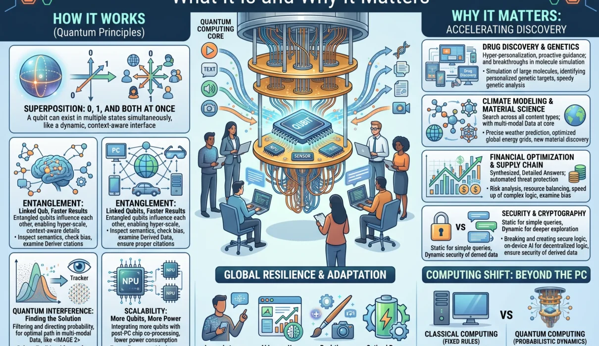
Rather than treating information as a series of binary switches, quantum computers leverage the fundamental laws of quantum mechanics: superposition, entanglement, and quantum interference. These machines do not simply process calculations faster; they calculate in fundamentally different mathematical spaces.
Understanding how quantum technology functions, why it delivers practical computational advantages, where its engineering limitations lie, and how it will reshape industries is critical for navigating the landscape of future computing.
CLASSICAL VS. QUANTUM COMPUTING: AT A GLANCE
┌────────────────────────────────────────────────────────────────────────┐
│ CLASSICAL COMPUTING                  QUANTUM COMPUTING                 │
│ • Unit: Binary Bit (0 OR 1)          • Unit: Quantum Bit / Qubit       │
│ • State: Deterministic voltage       • State: Complex superposition    │
│ • Scaling: Linear ($N$ bits = $N$ states) • Scaling: Exponential ($2^N$ states) │
│ • Interaction: Boolean logic gates   • Interaction: Unitary transforms │
│ • Core Mechanism: Step-by-step paths • Mechanism: Quantum interference │
└────────────────────────────────────────────────────────────────────────┘
1. What Is Quantum Computing? Moving Beyond Binary Logic
To grasp how quantum computing works, we must first examine the physics governing classical information.
In a classical microprocessor, a bit is a physical circuit that is either off ($0$) or on ($1$). If you have three classical bits, they can exist in one of $2^3 = 8$ possible configurations at any single instant:
$$\{000, 001, 010, 011, 100, 101, 110, 111\}$$
To evaluate which of those eight combinations solves a problem, a classical computer evaluates them sequentially or divides the work across multiple physical cores.
A qubit (quantum bit) behaves according to the laws of quantum mechanics. A qubit can represent a 0, a 1, or any quantum linear combination of both states simultaneously—a property known as superposition.
CLASSICAL BIT VS. QUANTUM QUBIT

Classical Bit:
[State: 0] ─────────────── OR ───────────────► [State: 1]
(A binary switch flipped completely to the north or south pole)

Quantum Qubit (The Bloch Sphere):
                 |0⟩ (North Pole)
                     ▲
                     │     ↗ |ψ⟩ (State Vector)
                     │   /
                     │ / θ (Polar angle)
           ──────────┼──────────►
                    /│ \ ϕ (Azimuthal phase)
                   / │  \
                  ↙  │   ▼
                 |1⟩ (South Pole)
(Any continuous coordinate across the entire spherical surface)
In mathematical terms, a qubit’s quantum state $\vert{}\psi\rangle$ is represented as a normalized vector on a unit sphere (known as the Bloch Sphere):
$$\vert{}\psi\rangle = \alpha\vert{}0\rangle + \beta\vert{}1\rangle$$
Here, $\alpha$ and $\beta$ are complex numbers representing probability amplitudes. When the qubit is measured, the delicate quantum state collapses into a classical outcome: it yields a 0 with probability $\vert{}\alpha\vert{}^2$ and a 1 with probability $\vert{}\beta\vert{}^2$, where:
$$\vert{}\alpha\vert{}^2 + \vert{}\beta\vert{}^2 = 1$$
When multiple qubits are combined, their computational capacity does not scale linearly ($1 + 1 = 2$); it scales exponentially.
While three classical bits hold one of eight combinations at a time, three entangled qubits in superposition hold all eight states simultaneously. A system of $N$ qubits can maintain a coherent superposition of $2^N$ states:
- 10 Qubits: 1,024 values in parallel
- 30 Qubits: Over 1 billion values in parallel
- 50 Qubits: Over 1.12 quadrillion values in parallel
- 300 Qubits: More simultaneous values than the estimated total number of atoms in the observable universe (~$10^{80}$)
A quantum computer does not execute instructions as a faster version of a silicon CPU. It acts as an advanced mathematical engine that manipulates multidimensional probability waves across an exponential configuration space.
2. The Core Mechanics: Superposition, Entanglement, and Interference
The computational power of quantum technology rests upon three physical phenomena: superposition, entanglement, and quantum interference.
THE THREE PILLARS OF QUANTUM MECHANICS IN COMPUTING

1. SUPERPOSITION: The State Space Multiplier
   Qubits inhabit continuous linear combinations of states, creating a
   $2^N$-dimensional Hilbert computational canvas.

2. ENTANGLEMENT: Non-Local Correlation
   Qubits link intrinsically; the state of one instantly dictates the state
   of another, eliminating classical communication overhead.

3. QUANTUM INTERFERENCE: The Algorithmic Sieve
   Constructive interference amplifies the correct mathematical answer;
   destructive interference cancels out billions of incorrect paths.
1. Superposition: The High-Dimensional State Canvas
In classical physics, an object occupies a single deterministic state: a coin sitting on a table shows either heads or tails.
Superposition is analogous to a coin spinning continuously on a tabletop: while spinning, it exhibits characteristics of both heads and tails simultaneously. The system contains the mathematical potential for both outcomes until an external measurement forces it to settle flat onto the table.
In a quantum processor, microwave pulses or laser beams place physical qubits into precise superposition angles, initializing an expansive computational workspace before calculations begin.
2. Entanglement: Non-Local Correlation
Albert Einstein famously referred to entanglement as “spooky action at a distance.” In quantum information science, it is the primary engine of non-classical computational scaling.
When two or more qubits become entangled, their physical states become inseparable. You can no longer describe the mathematical state of Qubit A without explicitly describing the state of Qubit B.
If two qubits are entangled in a Bell state:
$$\vert{}\Phi^+\rangle = \frac{1}{\sqrt{2}}(\vert{}00\rangle + \vert{}11\rangle)$$
Measuring Qubit A and finding it in state $0$ forces Qubit B to collapse into state $0$ instantly, regardless of the physical distance separating them. In a quantum computer, entanglement links qubits across the register, allowing a logic gate applied to a single qubit to dynamically alter the probability amplitudes across the entire interconnected quantum system.
3. Quantum Interference: Extracting the Signal
A common misconception is that a quantum computer simply runs every possible calculation in parallel and reads them all out at the end. If a quantum computer worked that way, it would be useless: measuring $N$ qubits in an equal superposition would simply collapse the system into a single, random classical outcome, providing no speedup over guessing.
The key to useful quantum computing is quantum interference.
QUANTUM INTERFERENCE: AMPLIFYING THE RIGHT ANSWER

Initial Superposition (Billions of potential computational pathways):
───/\───/\───/\───/\───/\───/\───/\───/\───/\───/\───/\───/\───

Phase Inversion & Amplification (Unitary Gate Transformations):
[Incorrect Solution Path A]  ──/\──
                                   ├── Destructive Cancellation ──► 0% Probability
[Incorrect Solution Path B]  ──\/──

[Correct Target Solution]    ──/\──
                                   ├── Constructive Addition    ──► ~100% Probability
[Target Amplitude Match]     ──/\──
Just like water or sound waves, quantum probability amplitudes have phases (positive, negative, or complex angles). Quantum algorithms (such as Shor’s algorithm for prime factorization or Grover’s search algorithm) are designed with mathematical gates that induce:
- Destructive Interference: The probability amplitudes of billions of incorrect answers are shifted out of phase, canceling each other out to zero.
- Constructive Interference: The probability amplitudes corresponding to the mathematically correct solution align in phase, reinforcing one another and rising toward a probability near 100%.
When the engineer finally measures the quantum register, the wave function collapses, revealing the correct solution with high statistical confidence.
3. The Physical Hardware: How to Build a Quantum Computer
Unlike classical computers, which converged on silicon CMOS transistors decades ago, the quantum computing industry is exploring several competing physical architectures.
Building a qubit requires isolating a quantum-mechanical system from all environmental noise while retaining the ability to manipulate its state via external controls.
THE LEADING QUANTUM PROCESSOR ARCHITECTURES

Superconducting Loops (Transmons):
┌───────────────────────────────┐
│ Josephson Junctions / Circuits│  • Fast gate speeds (nanoseconds)
│ Dilution Fridge (<15 mK)      │  • Advanced lithography scalability
│ Examples: IBM, Google, Rigetti│  • High sensitivity to thermal noise
└───────────────────────────────┘

Trapped Ion Systems:
┌───────────────────────────────┐
│ Charged Atoms in RF Vacuums   │  • Exceptional coherence times
│ Laser-Manipulated Gates       │  • All-to-all qubit connectivity
│ Examples: IonQ, Quantinuum    │  • Slower physical gate execution
└───────────────────────────────┘

Neutral Atom Arrays (Rydberg):
┌───────────────────────────────┐
│ Optical Tweezers / Laser Traps│  • High 2D/3D physical density
│ Neutral Rydberg Atoms         │  • Dynamic spatial reconfiguration
│ Examples: QuEra, Pasqal       │  • Fast-scaling physical qubit counts
└───────────────────────────────┘

Photonic Quantum Systems:
┌───────────────────────────────┐
│ Photons / Waveguides / Lasers │  • Room-temperature operations
│ Phase-Shift Beam Splitters    │  • High-speed fiber interoperability
│ Examples: Xanadu, PsiQuantum  │  • Probabilistic gate hurdles
└───────────────────────────────┘
1. Superconducting Transmon Qubits
The most widely deployed architecture—championed by IBM, Google, and Rigetti—constructs artificial atoms using superconducting electrical circuits.
- The Mechanism: Lithographically etched circuits of niobium or aluminum contain a Josephson Junction (a microscopic insulating barrier sandwiched between two superconductors). At ultra-cold temperatures, electrical resistance drops to zero, and the circuit oscillates as an anharmonic quantum LC resonator.
- The Environment: Superconducting chips must be housed inside multi-stage dilution refrigerators operating at 15 millikelvin (-273.135°C / -459.64°F)—temperatures colder than the vacuum of deep space. Thermal energy would otherwise excite the circuit, causing the quantum state to collapse instantly.
- Pros & Cons: Extremely fast gate execution speeds (10 to 100 nanoseconds) and mature semiconductor manufacturing pipelines, balanced by short coherence times (microseconds) and wiring bottlenecks inside cryogenic chambers.
2. Trapped Ion Systems
Pioneered by companies like IonQ and Quantinuum, trapped ion computers use individual charged atoms (typically Ytterbium or Barium) as pristine, identical qubits.
- The Mechanism: Ions are suspended in an ultra-high vacuum chamber using electromagnetic fields generated by Radio Frequency (RF) Paul traps. High-precision lasers cool the ions and manipulate their internal electronic and nuclear hyperfine spin states.
- Pros & Cons: Because every Ytterbium ion in the universe is physically identical, these systems exhibit near-perfect manufacturing uniformity, long coherence times (seconds to minutes), and all-to-all qubit connectivity. However, optical gate operations are orders of magnitude slower than superconducting circuits (microseconds to milliseconds).
3. Neutral Atom Arrays (Rydberg Systems)
A rapidly advancing architecture developed by firms like QuEra and Pasqal suspends uncharged, neutral atoms (such as Rubidium or Cesium) in 2D and 3D geometric grids using focused laser beams called optical tweezers.
- The Mechanism: Lasers dynamically reposition individual atoms in real time. To execute a logic gate, specific atoms are excited into high-energy Rydberg states, expanding their electron clouds until they interact across multi-micrometer distances via the “Rydberg blockade” effect.
- Pros & Cons: Excellent scalability (arrays scaling past hundreds of physical atoms), reconfigurable connectivity, and long coherence times, though laser-pointing stability and cooling physics remain active engineering frontiers.
4. Photonic Quantum Computing
Championed by Xanadu and PsiQuantum, this architecture uses individual photons (particles of light) as qubits.
- The Mechanism: Quantum information is encoded into the polarization, spatial mode, or time-bin of photons generated by on-chip lasers. Computation occurs as light travels through optical waveguides, directional couplers, and phase shifters etched onto silicon photonic chips.
- Pros & Cons: Photons do not interact with ambient heat, allowing the primary optical processing matrix to run at room temperature. Photonic systems interface natively with fiber-optic telecom networks. However, because photons do not naturally interact with one another, executing two-qubit logic gates requires complex probabilistic measurements and high physical resource overhead.
4. The Engineering Bottleneck: Decoherence and Quantum Error Correction
The primary challenge preventing quantum computers from instantly taking over global computing is not building qubits; it is protecting them from noise.
Qubits are fragile. The slightest environmental vibration, thermal fluctuation, stray magnetic field, or cosmic ray can cause a qubit to lose its quantum-mechanical properties—a failure mode known as quantum decoherence.
DECOHERENCE AND THE NOISY INTERMEDIATE-SCALE QUANTUM (NISQ) WALL

Perfect Computational State:
|ψ⟩ = α|0⟩ + β|1⟩  ──► (Maintains phase and amplitude throughout algorithm)

Environmental Perturbation (Thermal noise, RF bleed, magnetic drift):
         │
         ▼
State Collapse / Decoherence:
|ψ⟩ ──► Phase Flip (Z-error) OR Bit Flip (X-error) ──► Random Classical Noise
The Transition: From Physical Qubits to Logical Qubits
For years, the quantum industry operated in the Noisy Intermediate-Scale Quantum (NISQ) era. In NISQ devices, algorithms run directly on bare, error-prone physical qubits.
Because physical gate error rates hover between $0.1\%$ and $1\%$, running an algorithm with more than a few dozen sequential operations causes errors to compound exponentially, drowning the true signal in random noise.
To achieve fault-tolerant computation, the industry is transitioning to Quantum Error Correction (QEC) and the creation of logical qubits.
PHYSICAL QUBIT OVERHEAD: CREATING A FAULT-TOLERANT LOGICAL QUBIT

┌────────────────────────────────────────────────────────────────────────┐
│ ONE STABLE LOGICAL QUBIT (Protected Quantum Data)                     │
├────────────────────────────────────────────────────────────────────────┤
│ Encoded across a topological surface code lattice:                     │
│                                                                        │
│   [P] ─── (A) ─── [P] ─── (A) ─── [P]       [P] = Data Physical Qubit │
│    │       │       │       │       │                                  │
│   (A) ─── [P] ─── (A) ─── [P] ─── (A)       (A) = Syndrome Ancilla    │
│    │       │       │       │       │             Qubit (Measures      │
│   [P] ─── (A) ─── [P] ─── (A) ─── [P]             Parity / Errors)    │
│                                                                        │
│ Continuous non-destructive stabilizer syndrome measurements detect     │
│ and correct bit-flips (X) and phase-flips (Z) in real time.            │
└────────────────────────────────────────────────────────────────────────┘
A logical qubit is a single, error-protected unit of quantum information distributed across a topological lattice of many physical qubits using error-correcting codes (such as surface codes or Quantum Low-Density Parity-Check / QLDPC codes):
- Data Qubits: Store the actual computational superposition state.
- Ancilla (Syndrome) Qubits: Interleaved across the lattice to perform non-destructive parity measurements. They detect whether a neighboring data qubit suffered a bit-flip or phase-flip error without measuring the data qubit directly, preserving the underlying superposition.
- The Scaling Tipping Point: A major milestone in quantum engineering is demonstrating below-threshold error suppression—proving that as you increase the size of the physical qubit lattice, the net logical error rate decreases exponentially rather than amplifying. Systems demonstrated by Google (Willow), Quantinuum, Harvard/QuEra, and IBM have verified that fault-tolerant scaling curves operate as theoretical physics predicted.
5. Quantum Advantage: What Can Quantum Computers Actually Solve?
Another common misconception is that quantum computers will replace classical PCs, making video games render instantly and web browsers load faster.
They will not. For everyday sequential computing, word processing, database lookups, and operating system management, classical architectures are faster, cheaper, and more reliable.
Quantum computers excel at mathematical classes that exhibit specific structural profiles: high-dimensional complexity with compact input/output requirements.
COMPUTATIONAL COMPLEXITY CLASSES
┌────────────────────────────────────────────────────────────────────────┐
│ P (Polynomial Time): Solved efficiently by classical computers         │
│ • Arithmetic, sorting, basic database queries                          │
│                                                                        │
│ BQP (Bounded-Error Quantum Polynomial Time):                           │
│ Problems solved efficiently by a quantum computer                      │
│ ┌────────────────────────────────────────────────────────────────────┐ │
│ │ • Quantum Simulation (Feynman)                                     │ │
│ │ • Prime Factorization (Shor's Algorithm)                           │ │
│ │ • Discrete Logarithms & Elliptic Curves                            │ │
│ └────────────────────────────────────────────────────────────────────┘ │
│                                                                        │
│ NP-Complete / Hard:                                                    │
│ • Traveling Salesperson, General Combinatorial Optimization           │
│ (Quantum provides quadratic Grover speedups or heuristic advantages,  │
│  not instant polynomial magic solutions)                              │
└────────────────────────────────────────────────────────────────────────┘
1. Simulating Quantum Chemistry and Materials Science
As the physicist Richard Feynman noted in 1981:
“Nature isn’t classical, dammit, and if you want to make a simulation of nature, you’d better make it quantum mechanical.”
Because electrons interacting inside molecules are quantum systems, classical computers must approximate their wavefunctions using severe mathematical simplifications. A classical supercomputer struggles to accurately model a caffeine molecule ($C_8H_{10}N_4O_2$); it cannot accurately simulate the active catalytic center of nitrogenase (FeMoco)—the bacterial enzyme that fixes nitrogen at ambient temperatures and pressures.
THE NITROGEN FIXATION REVOLUTION

Classical Problem:
The industrial Haber-Bosch process manufactures synthetic fertilizer by breaking
atmospheric nitrogen bonds at extreme temperatures (450°C) and pressure (200 atm).
Consumes 1% to 2% of the entire planet's annual energy supply.

Quantum Solution:
A fault-tolerant quantum computer simulates the FeMoco enzyme's catalytic transition
states, identifying room-temperature, ambient-pressure bio-catalysts.
Slashing global industrial energy consumption by gigawatt-hours.
- Pharmaceutical Discovery: Simulating exact drug-target protein binding affinities in days, replacing years of trial-and-error laboratory wet-chemistry synthesis.
- Next-Generation Batteries: Modeling solid-state electrolyte interfaces, lithium-dendrite formation, and novel cathode chemistries to increase energy density by 300%.
- Room-Temperature Superconductors: Simulating electron-phonon interactions to design materials that transport electricity with zero loss without cryogenic cooling.
2. High-Dimensional Optimization and Logistics
Global supply chains, airline route scheduling, telecommunications traffic management, and portfolio risk modeling are examples of combinatorial optimization. As variables increase, the number of possible routing combinations explodes exponentially.
Quantum algorithms—such as the Quantum Approximate Optimization Algorithm (QAOA) and quantum annealing—explore complex, multi-peaked energy landscapes:
- Rather than climbing over high mathematical barriers, quantum systems can “tunnel” through energy barriers (quantum tunneling) to discover global cost minima faster than classical heuristics.
- Optimizing dynamic maritime container routing to cut fuel consumption and carbon emissions across global shipping fleets.
3. Financial Portfolio Modeling and Arbitrage
Financial markets generate multi-dimensional risk matrices with millions of correlated assets:
- Quantum Monte Carlo Acceleration: Pricing complex derivative instruments and evaluating systemic liquidity shock risks. While classical Monte Carlo simulations scale as $O(1/\epsilon^2)$ with precision $\epsilon$, quantum amplitude estimation algorithms scale quadratically faster as $O(1/\epsilon)$, turning overnight risk computations into near-real-time trading decisions.
6. The Cybersecurity Paradigm Shift: Shor’s Algorithm and Post-Quantum Cryptography
The most urgent real-world application of quantum computing is not scientific discovery—it is cybersecurity.
Modern digital commerce and internet communications are secured by public-key asymmetric cryptography: RSA, Diffie-Hellman, and Elliptic Curve Cryptography (ECC). These systems protect everything from bank wire transfers and military communications to secure web traffic (HTTPS) and blockchain networks.
THE RSA ASYMMETRIC SECURITY CRACK

The Classical Defense:
Multiplying two large prime numbers ($p \times q = N$) takes milliseconds.
Factoring the product ($N$) back into its prime factors takes classical
supercomputers thousands of years via the General Number Field Sieve (GNFS).

The Quantum Offensive (Shor's Algorithm):
1. In 1994, Peter Shor demonstrated that a fault-tolerant quantum computer
   solves prime factorization in Polynomial Time: $O((\log N)^3)$.
2. Transforms an intractable, multi-millennium calculation into an operation
   resolved in hours or days.
3. RSA-2048 and ECC-256 are rendered cryptographically broken.
The Immediate Threat: “Store Now, Decrypt Later” (SNDL)
You might assume that because large-scale fault-tolerant quantum computers capable of breaking RSA-2048 are still years away, post-quantum risks can wait.
This assumption is dangerously flawed.
Hostile nation-states and cybercrime syndicates are actively executing Store Now, Decrypt Later (SNDL) campaigns:
- Adversaries intercept and harvest encrypted enterprise communications, diplomatic cables, trade secrets, intellectual property, and medical histories off global fiber backbones today.
- They store this encrypted data in storage arrays.
- The moment a cryptanalytically relevant quantum computer (CRQC) becomes operational, that archived data will be decrypted retroactively. If your enterprise data must remain secret for 10, 20, or 30 years, it is vulnerable right now.
                THE "STORE NOW, DECRYPT LATER" (SNDL) ATTACK TIMELINE

  PRESENT DAY:                                    FUTURE (Q-Day):
  ┌───────────────────────────┐                   ┌───────────────────────────┐
  │ Intercept & Exfiltrate    │                   │ Large-Scale Quantum       │
  │ Encrypted Traffic Today   │ ──(Stored in Data ──► Computer Executes       │
  │ (Protected by RSA/ECC)    │    Warehouses)    │ Shor's Algorithm          │
  └───────────────────────────┘                   └─────────────┬─────────────┘
                                                                │
                                                                ▼
                                                  Plaintext Data Exposed:
                                                  • Trade secrets & IP
                                                  • Government communications
                                                  • Historical patient records
The Global Defense: Post-Quantum Cryptography (PQC)
To counter the quantum threat, the National Institute of Standards and Technology (NIST) conducted an eight-year global competition to develop Post-Quantum Cryptography (PQC)—mathematical algorithms that run on standard classical computers but are resistant to attacks from both classical and quantum computers.
┌────────────────────────────────────────────────────────────────────────┐
│                   NIST POST-QUANTUM CRYPTOGRAPHY STANDARDS             │
├─────────────────────┬────────────────────┬─────────────────────────────┤
│ Standard Algorithm  │ Mathematical Basis │ Primary Replacement Target  │
├─────────────────────┼────────────────────┼─────────────────────────────┤
│ ML-KEM              │ Module-Lattice     │ Replaces RSA & Diffie-      │
│ (FIPS 203)          │ Cryptography       │ Hellman Key Exchange        │
├─────────────────────┼────────────────────┼─────────────────────────────┤
│ ML-DSA              │ Module-Lattice     │ Replaces RSA & ECDSA        │
│ (FIPS 204)          │ Digital Signatures │ Digital Identity Signatures │
├─────────────────────┼────────────────────┼─────────────────────────────┤
│ SLH-DSA             │ Stateless Hash-    │ High-Assurance Backup       │
│ (FIPS 205)          │ Based Signatures   │ Digital Signature Scheme    │
└─────────────────────┴────────────────────┴─────────────────────────────┘
These standards replace factoring-based math with complex mathematical lattices (the Shortest Vector Problem in high-dimensional vector grids). Even with Shor’s algorithm, a quantum computer cannot search lattice spaces in polynomial time.
Migrating global infrastructure to PQC standards is the most urgent cybersecurity mandate of the current decade.
7. The 2026 Landscape: Where Does the Technology Stand Today?
We have exited the era of purely theoretical laboratory physics. In 2026, quantum computing has officially entered the era of quantum industrialization and hybrid deployment.
THE COMPUTATIONAL TIMELINE

Pre-2024: Pure Science & NISQ Demonstrations
• Proof-of-concept chips with high error rates (50–100 noisy physical qubits).
• "Quantum Supremacy" claims on esoteric, non-practical sampling tasks.

2025–2026: The Inflection Point of Verified Advantage
• Logical qubits scale into the dozens and hundreds.
• Verified below-threshold error correction demonstrated across multiple architectures.
• Practical hybrid quantum-classical workflows deploy in enterprise pilots.

Late 2020s (2028–2030): Fault-Tolerant Utility
• Systems operating 1,000+ stable logical qubits with active QEC.
• First commercial discoveries in molecular chemistry and materials design.

2030s: Full Industrial Scale
• Universal fault-tolerant quantum computing commoditized across cloud backbones.
• Cryptanalytic capability reaches Shor's algorithm thresholds; classical RSA retired.
The Hybrid Quantum-Classical Operating Model
Enterprises are not waiting for million-qubit machines to extract value. The production architecture of 2026 is hybrid quantum-classical orchestration:
- Classical high-performance compute (HPC) clusters manage data pre-processing, operating systems, and linear algebra baselines.
- Specific, computationally intractable sub-routines (e.g., estimating an intractable molecular ground-state energy or optimizing a sub-graph) are packaged as quantum circuits and dispatched to a cloud-hosted Quantum Processing Unit (QPU).
- The QPU executes the circuit, performs error suppression, and returns the result to the classical pipeline.
Supported by Quantum-as-a-Service (QaaS) platforms across AWS Braket, Microsoft Azure Quantum, Google Quantum AI, and IBM Quantum Network, organizations can build, test, and benchmark hybrid workflows using Python libraries (Qiskit, Cirq, PennyLane) without owning physical cryostats.
8. Summary Comparison: Classical vs. Quantum Computing
To synthesize how these paradigms diverge across every layer of the computing stack:
| Parameter | Classical Supercomputing | Quantum Computing (Fault-Tolerant) |
| Fundamental Unit | Classical Bit (0 or 1) | Quantum Bit / Qubit ($\vert{}\psi\rangle = \alpha\vert{}0\rangle + \beta\vert{}1\rangle$) |
| Physical Implementation | Silicon CMOS Field-Effect Transistors | Superconducting circuits, trapped ions, neutral atoms, photons |
| Operating Temperature | Ambient to Air/Liquid Cooled (~20°C to 50°C) | Deep Cryogenic (~0.015 Kelvin) or optical room temperature |
| Mathematical Logic | Boolean Gates (AND, OR, NOT, NAND) | Reversible Unitary Operators (Hadamard, CNOT, Phase, T-gates) |
| Scaling Function | Linear / Polynomial Scaling ($N$) | Exponential State-Space Capacity ($2^N$) |
| Error Handling | Parity checks, ECC memory (Rare bit-flips) | Active Quantum Error Correction (Surface codes, QLDPC) |
| Primary Use Cases | General software, web services, machine learning, standard physics | Molecular simulation, prime factorization, combinatorial optimization, quantum physics |
| Data Output | Exact deterministic value or fixed float | Probabilistic measurement collapsed via wave interference |
9. Strategic Action Plan: How Technical Leaders Must Prepare
Quantum computing is no longer a science project confined to university physics departments. It is a strategic capability that requires proactive organizational preparation.
┌────────────────────────────────────────────────────────────────────────┐
│               ENTERPRISE QUANTUM READINESS ROADMAP                     │
├─────────────────────┬──────────────────────────────────────────────────┤
│ Strategic Horizon   │ Immediate Tactical Priority                      │
├─────────────────────┼──────────────────────────────────────────────────┤
│ Step 1: Crypto-     │ Audit all enterprise cryptographic assets; map   │
│ Agility Audit       │ where RSA and ECC are deployed across databases, │
│                     │ APIs, and VPN endpoints.                         │
├─────────────────────┼──────────────────────────────────────────────────┤
│ Step 2: Implement   │ Begin phased migration to NIST PQC standards     │
│ PQC Algorithms      │ (ML-KEM, ML-DSA) on high-value data channels.    │
├─────────────────────┼──────────────────────────────────────────────────┤
│ Step 3: Identify    │ Pinpoint company bottlenecks: Is it molecular    │
│ High-Value Use Cases│ chemistry, complex logistics, or risk pricing?   │
├─────────────────────┼──────────────────────────────────────────────────┤
│ Step 4: Cultivate   │ Train internal teams on hybrid quantum SDKs      │
│ Quantum Fluency     │ (Qiskit, Cirq); pilot cloud QaaS integrations.   │
└─────────────────────┴──────────────────────────────────────────────────┘
- Establish Cryptographic Agility Immediately: The most pressing quantum action item does not require buying a quantum computer. Audit your enterprise infrastructure for legacy public-key algorithms. Design your software architecture to be crypto-agile—ensuring that underlying encryption algorithms (TLS certificates, SSH keys, database encryption) can be swapped out for NIST-approved Post-Quantum Cryptography standards without rewriting application code.
- Identify Your Quantum Bottlenecks: Evaluate your operational problems. Does your company spend millions of dollars running approximate classical simulations for materials design, fluid dynamics, or logistical scheduling? Identify the mathematical problems in your business that fit into bounded-error quantum polynomial time (BQP) profiles.
- Upskill and Pilot via Cloud QaaS: Do not wait for fault-tolerant hardware to train your engineering teams. Use cloud-accessible quantum platforms to experiment with quantum algorithms. Build hybrid pipelines that integrate classical data warehouses with quantum processors, developing the institutional fluency required to leverage quantum advantage the moment the hardware fully scales.
The New Frontier of Human Computation
For thousands of years, computing was tied to physical tallies: pebbles in the sand, gears in an abacus, punch cards in a mechanical loom, and electric charges running through silicon traces. Yet every one of those machines operated under the same classical assumptions of cause and effect that govern our macroscopic daily lives.
Quantum computing breaks that historical continuity.
By building machines that operate according to the fundamental laws of the subatomic universe, humanity is accessing an entirely new computational realm.
Quantum computing will not replace classical computers. It will stand alongside them: classical processors will continue managing the human-facing digital world, while quantum processors quietly resolve the fundamental molecular, energetic, and mathematical problems that have constrained scientific progress for centuries.
From designing zero-carbon industrial catalysts and curing complex diseases to unravelling the deepest mysteries of physics, quantum computing represents more than faster processing. It is the technological key that unlocks nature’s computational operating system.